
Machine learning fundamentals, for genomics researchers#

This notebook uses cell-type classification as a running example for concepts that apply to supervised machine learning in general. No prior machine learning is assumed. By the end, you will be able to:
interpret a model’s outputs and its loss,
follow one gradient update from start to finish, and
use training, validation, and test data to recognize overfitting.
The data here is deliberately synthetic, which keeps the focus on the mechanics rather than on any particular biology. The applied tutorial runs this same training loop on a real AnnData dataset.
import copy

import matplotlib.pyplot as plt
import numpy as np
import torch
import torch.nn as nn

%matplotlib inline

SEED = 0
rng = np.random.default_rng(SEED)
torch.manual_seed(SEED)
print("CHECKPOINT 1/3 - Setup complete")
CHECKPOINT 1/3 - Setup complete
1. From data points to tensors#
A supervised dataset contains data points (also called examples or observations). Each data point has an input \(x\) made up of measured features, and a target \(y\) we want to predict. A data point could be an image, a patient, a molecule, or any object represented by numbers.
For \(n\) data points with \(p\) features each, the inputs are arranged in a matrix \(X \in \mathbb{R}^{n \times p}\), one row per data point, and the targets in a vector \(y\) with one entry per row.
In our running example a data point is a cell, its features are gene-expression values, and its target is a cell type. We use simulated data to keep things self-contained (the values stand in for standardized or log-transformed expression, not raw counts): each of three cell types has a characteristic average profile, and individual cells vary around it.
n_genes, n_types = 200, 3
profiles = rng.normal(size=(n_types, n_genes)) * 0.15


def sample_cells(n_per_type):
    X = np.concatenate([
        rng.normal(size=(n_per_type, n_genes)) + profiles[cell_type]
        for cell_type in range(n_types)
    ])
    y = np.repeat(np.arange(n_types), n_per_type)
    return torch.tensor(X, dtype=torch.float32), torch.tensor(y, dtype=torch.long)
We first generate one small, balanced dataset and use it as a whole. At this stage the goal is to understand tensors, model outputs, losses, and parameter updates, so we deliberately postpone train/validation/test splitting until generalization becomes the question.
The function returns a feature matrix \(X\) and a target vector \(y\).
X, y = sample_cells(n_per_type=30)
PyTorch represents data with tensors, general-purpose multidimensional arrays similar to NumPy arrays. A tensor’s shape records the size of each axis. For a feature matrix, the first axis indexes data points and the second indexes features.
print("features:", X.shape, X.dtype)
print("labels:  ", y.shape, y.dtype)
print("data points per class:", torch.bincount(y))
print(f"CHECKPOINT 2/3 - Data ready: {X.shape[0]} cells x {X.shape[1]} features")
features: torch.Size([90, 200]) torch.float32
labels:   torch.Size([90]) torch.int64
data points per class: tensor([30, 30, 30])
CHECKPOINT 2/3 - Data ready: 90 cells x 200 features
X has one row per data point (cell) and one column per feature (gene). y holds one integer class label per row. That is all the structure the model needs.
2. A model maps inputs to outputs#
A model is a function \(f(x; \theta)\) that maps one data point \(x\) to an output. The meaning of the output depends on the task: it could be a number for regression or a set of class scores for classification. The parameters \(\theta\) are internal values learned from data, such as weights and biases.
We begin with a linear model,
where \(\theta = \{W, b\}\). In our running example, \(x\) is one cell’s 200-dimensional expression vector, and the output \(f(x; \theta)\) is three scores, one per cell type.
linear_model = nn.Linear(in_features=n_genes, out_features=n_types)

n_parameters = sum(parameter.numel() for parameter in linear_model.parameters())
print(linear_model)
print(f"trainable parameters: {n_parameters}")
Linear(in_features=200, out_features=3, bias=True)
trainable parameters: 603
A forward pass sends input through the model to produce an output using the current parameters. It does not change them. Calling the model runs it.
For classification, the model outputs one score per class. Passing six cells through it gives six rows, one column per cell type. The higher a class’s score, the more the model favours that class.
example_idx = torch.tensor([0, 30, 60, 1, 31, 61])
example_X = X[example_idx]
example_y = y[example_idx]
example_scores = linear_model(example_X)

print("input shape: ", example_X.shape)
print("output shape:", example_scores.shape)
print("first cell's class scores:", example_scores[0].detach())
input shape:  torch.Size([6, 200])
output shape: torch.Size([6, 3])
first cell's class scores: tensor([-0.7742, -0.0423,  0.4269])
The predicted class is the one with the largest score. To read the scores as probabilities, softmax turns them into positive numbers that sum to one. That is handy for interpretation, though the loss below works straight from the raw scores.
example_probabilities = torch.softmax(example_scores, dim=1)
example_predictions = example_scores.argmax(dim=1)

print("probabilities for first cell:", example_probabilities[0].detach())
print("predicted classes:           ", example_predictions)
print("true classes:                ", example_y)
probabilities for first cell: tensor([0.1562, 0.3247, 0.5191])
predicted classes:            tensor([2, 0, 1, 2, 1, 0])
true classes:                 tensor([0, 1, 2, 0, 1, 2])
3. A loss scores the predictions#
A loss function measures how far the model’s outputs are from the targets: high when predictions are wrong, low when they are right. Training adjusts the parameters to make the average loss over the training data, written \(\mathcal{L}(\theta)\), as small as possible.
Which loss to use depends on the task. Mean squared error is common for regression. For classification we use cross-entropy, which rewards putting high probability on the correct class. nn.CrossEntropyLoss takes the raw class scores and the integer labels (0, 1, 2) directly, and applies the softmax internally so you don’t add one yourself.
loss_fn = nn.CrossEntropyLoss()
example_loss = loss_fn(example_scores, example_y)
print(f"cross-entropy loss: {example_loss.item():.3f}")
cross-entropy loss: 1.648
4. One gradient-descent step#
Optimization is the process of changing model parameters to reduce the loss. The gradient \(\nabla_\theta \mathcal{L}\) is the collection of partial derivatives of the loss with respect to every parameter. It describes the loss’s local sensitivity and points toward the steepest local increase.
Gradient descent therefore takes a step in the opposite direction:
where the learning rate \(\eta\) controls the step size. A real model has many parameters. This illustration shows the same idea with only two.
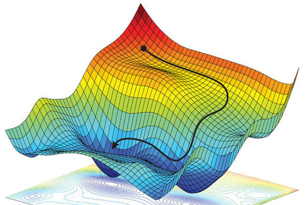
During the forward pass, PyTorch records how tensors were combined in a computation graph. Calling loss.backward() applies the chain rule backward through that graph and stores a gradient in the .grad attribute of every trainable parameter.
optimizer = torch.optim.SGD(linear_model.parameters(), lr=0.1)
optimizer.zero_grad()
loss_before = loss_fn(linear_model(X), y)
loss_before.backward()

print("weight gradient shape:", linear_model.weight.grad.shape)
print(f"weight gradient norm: {linear_model.weight.grad.norm().item():.3f}")
weight gradient shape: torch.Size([3, 200])
weight gradient norm: 1.769
PyTorch accumulates gradients by default, which is useful in some advanced workflows. Here each update should use only the current calculation, so zero_grad() clears gradients left by the previous step before backward() calculates new ones.
optimizer.step()

with torch.no_grad():
    loss_after = loss_fn(linear_model(X), y)

print(f"loss before update: {loss_before.item():.3f}")
print(f"loss after update:  {loss_after.item():.3f}")
loss before update: 1.309
loss after update:  1.018
For this model, dataset, and learning rate, the update lowered the loss. More generally, a gradient step tries to lower the loss using local information. A learning rate that is too large can overshoot and make an individual step increase the loss instead.
5. The training loop#
A training step consists of clearing old gradients, running a forward pass, calculating the loss and gradients, and updating the parameters. Training repeats this step many times. An epoch is one complete pass through the training data.
We reinitialize the linear model so the run starts from a reproducible state. Each step below uses all 90 data points at once, so one epoch is a single update. This is full-batch gradient descent, which keeps the mechanics simple. (Larger datasets are trained in smaller mini-batches instead, which the next tutorial does.)
linear_model = nn.Linear(n_genes, n_types)
optimizer = torch.optim.SGD(linear_model.parameters(), lr=0.1)
linear_losses = []

for epoch in range(50):
    linear_model.train()
    optimizer.zero_grad()
    loss = loss_fn(linear_model(X), y)
    loss.backward()
    optimizer.step()
    linear_losses.append(loss.item())
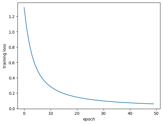
A learning curve plots a measured quantity against training time. Here we plot loss after each epoch to make the optimization process visible. Its exact shape depends on the data, initialization, optimizer, and learning rate, but successful training should reduce it overall.
plt.plot(linear_losses)
plt.xlabel("epoch")
plt.ylabel("training loss")
plt.show()
Evaluation#
Evaluation measures a trained model without updating it. model.eval() switches the model into evaluation mode, and torch.no_grad() skips the gradient bookkeeping that is only needed for training. The small helper below uses both to compute accuracy.
def accuracy(model, X, y):
    model.eval()
    with torch.no_grad():
        predictions = model(X).argmax(dim=1)
    return (predictions == y).float().mean().item()
print(f"accuracy on the data used for training: {accuracy(linear_model, X, y):.2f}")
accuracy on the data used for training: 1.00
6. Training performance is not generalization#
The accuracy above was measured on the very same cells the model trained on, so of course it looks good. What we actually care about is how the model does on new cells it has never seen, and the two can come apart.
That gap tends to open up when a model has a lot of capacity: the flexibility to fit many different patterns. Capacity is double-edged. It lets a model capture real structure, but it also lets it latch onto accidental quirks of the particular cells it trained on. Fitting those quirks is overfitting: the training score keeps improving while performance on new cells stalls or gets worse.
To make overfitting easy to see, we swap the linear model for something with more capacity: a multilayer perceptron (MLP). It stacks two linear layers with a simple nonlinear step in between (ReLU, which just replaces negative values with zero), letting it represent more flexible decision boundaries than a single linear layer can.
class MLP(nn.Module):
    def __init__(self, n_in, n_out, n_hidden=64):
        super().__init__()
        self.net = nn.Sequential(
            nn.Linear(n_in, n_hidden),
            nn.ReLU(),
            nn.Linear(n_hidden, n_out),
        )

    def forward(self, x):
        return self.net(x)
mlp = MLP(n_genes, n_types)
linear_count = sum(p.numel() for p in linear_model.parameters())
mlp_count = sum(p.numel() for p in mlp.parameters())
print(f"linear model parameters: {linear_count:,}")
print(f"MLP parameters:          {mlp_count:,}")
linear model parameters: 603
MLP parameters:          13,059
To measure generalization, we now begin a fresh experiment and split one new dataset into disjoint parts:
the training set supplies parameter updates,
the validation set guides choices such as early stopping, and
the test set is reserved for the final evaluation.
We use scikit-learn’s train_test_split, with stratify=y to preserve the class proportions in every split. Only five percent of the data becomes the training set. That is deliberately small, because a tiny training set paired with a high-capacity model is the easy way to see overfitting. In real projects the training set is normally the largest split. The rest is divided equally between validation and test. With overlapping classes, 200 features, and only 90 training points, the MLP has plenty of room to memorize.
# train_test_split gives a stratified split (equal class proportions) in one line.
# PyTorch's random_split is unstratified and works on Datasets, not raw tensors, so we use sklearn here.
from sklearn.model_selection import train_test_split

X_all, y_all = sample_cells(n_per_type=600)
train_fraction = 0.05

X_train, X_held_out, y_train, y_held_out = train_test_split(
    X_all,
    y_all,
    train_size=train_fraction,
    stratify=y_all,
    random_state=SEED,
)
X_val, X_test, y_val, y_test = train_test_split(
    X_held_out,
    y_held_out,
    train_size=0.5,
    stratify=y_held_out,
    random_state=SEED,
)

print("split sizes:", len(X_train), len(X_val), len(X_test))
print("training points per class:", torch.bincount(y_train))
print(f"MLP parameters per training point: {mlp_count / len(X_train):.1f}")
split sizes: 90 855 855
training points per class: tensor([30, 30, 30])
MLP parameters per training point: 145.1
7. Validation detects overfitting#
If we only ever watch the training loss, we can’t tell learning from memorizing, since it keeps dropping either way. The fix is to hold out a validation set: cells the model is scored on but never trains on. That gives an honest progress signal we can act on (model selection). Here we use it simply: keep the version of the model from the epoch with the lowest validation loss, a basic form of early stopping.
We first evaluate the untrained model on both the training and validation cells; this is epoch 0. We then train the MLP, evaluate both sets again after every epoch, and leave the test set untouched until the very end. (We also switch the optimizer from SGD to Adam, which adjusts the step size for each parameter automatically. The loop is otherwise identical: zero_grad(), backward(), step() play the same roles.)
# reuse the mlp we defined above, which has not been trained yet
optimizer = torch.optim.Adam(mlp.parameters(), lr=0.002)

mlp.eval()
with torch.no_grad():
    train_losses = [loss_fn(mlp(X_train), y_train).item()]
    val_losses = [loss_fn(mlp(X_val), y_val).item()]

best_val_loss = val_losses[0]
best_state = copy.deepcopy(mlp.state_dict())
Epoch 0 records both losses before any parameter updates. After each training epoch, we switch to evaluation mode and calculate both losses again without gradients, so the curves compare the same model state. Whenever validation loss reaches a new minimum, we save a copy of the current parameters. Validation affects which parameters we keep, but it never supplies a training gradient.
for epoch in range(300):
    mlp.train()
    optimizer.zero_grad()
    train_loss = loss_fn(mlp(X_train), y_train)
    train_loss.backward()
    optimizer.step()

    mlp.eval()
    with torch.no_grad():
        train_losses.append(loss_fn(mlp(X_train), y_train).item())
        val_losses.append(loss_fn(mlp(X_val), y_val).item())

    if val_losses[-1] < best_val_loss:
        best_val_loss = val_losses[-1]
        best_state = copy.deepcopy(mlp.state_dict())

best_epoch = int(np.argmin(val_losses))
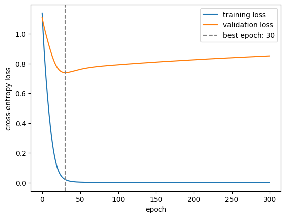
This is the characteristic pattern of overfitting: training loss keeps falling toward zero, while validation loss reaches a minimum and then rises. With continued training, the MLP becomes increasingly confident about patterns specific to the small training sample. The validation minimum identifies an earlier model without consulting the test set.
epochs = np.arange(len(train_losses))
plt.plot(epochs, train_losses, label="training loss")
plt.plot(epochs, val_losses, label="validation loss")
plt.axvline(best_epoch, color="gray", linestyle="--", label=f"best epoch: {best_epoch}")
plt.xlabel("epoch")
plt.ylabel("cross-entropy loss")
plt.legend()
plt.show()
The test set is used only after training and model selection are complete. Here we report both cross-entropy and accuracy for the final model and the validation-selected model. Accuracy records only whether the largest score names the correct class. Cross-entropy also measures how much probability the model assigns to that class, so it can reveal increasingly confident mistakes even when accuracy changes little.
best_mlp = MLP(n_genes, n_types)
best_mlp.load_state_dict(best_state)
mlp.eval()
best_mlp.eval()
with torch.no_grad():
    final_test_loss = loss_fn(mlp(X_test), y_test).item()
    selected_test_loss = loss_fn(best_mlp(X_test), y_test).item()

print(f"training accuracy after 300 epochs: {accuracy(mlp, X_train, y_train):.2f}")
print(f"lowest validation loss at epoch:    {best_epoch}")
print()
print(f"test cross-entropy, final model:    {final_test_loss:.3f}")
print(f"test cross-entropy, selected model: {selected_test_loss:.3f}")
print(f"test accuracy, final model:         {accuracy(mlp, X_test, y_test):.2f}")
print(f"test accuracy, selected model:      {accuracy(best_mlp, X_test, y_test):.2f}")
print("CHECKPOINT 3/3 - Model trained and evaluated")
training accuracy after 300 epochs: 1.00
lowest validation loss at epoch:    30

test cross-entropy, final model:    0.739
test cross-entropy, selected model: 0.681
test accuracy, final model:         0.71
test accuracy, selected model:      0.72
CHECKPOINT 3/3 - Model trained and evaluated
8. The complete picture#
The validation-selected model has lower test cross-entropy than the model trained for all 300 epochs. This confirms that prolonged training overfit ordinary sample variation even though every training label was correct. The rounded test accuracies can stay similar because accuracy ignores changes in confidence that do not flip the winning class. Both sit near 0.71, well above the 0.33 chance level for three balanced classes.
More generally, supervised data points are represented by features and paired with targets. A parameterized model maps features to outputs, a loss measures how far those outputs are from the targets, and its average \(\mathcal{L}(\theta)\) over the training data guides parameter updates. Training performance describes fit to known examples. Validation data guide model choices, and test data estimate generalization.
Cell-type classification supplied the concrete data here, but the same structure applies to other classification and regression problems. The applied PyTorch tutorial builds on this loop with Dataset and DataLoader objects for larger AnnData collections and mini-batch training.