Single-cell data in PyTorch

This notebook shows how to feed a single-cell dataset, stored as an AnnData object, into a PyTorch model. The fundamentals notebook built the training loop from scratch, so here we focus on the part that is specific to single-cell data: turning an AnnData object into the batches of tensors a training loop consumes.

We use the common case, where one cell is one training example, with anndata’s own AnnLoader. Two examples show the pattern: predicting a cell’s type (a classification) and predicting a continuous property of a cell (a regression). Only the target column changes between them. A follow-up tutorial handles the case where one example is a whole patient.

Setup

On Google Colab, run the install cell once. The data loader below downloads the dataset (about 1.9 GB) the first time and caches it under ../data/, the same file the basics notebook uses.

import IPython

# Setup environment: run this cell once.
try:
    import numpy as np
    import torch
    import scanpy as sc
    import ggml_ot
    from anndata.experimental import AnnLoader
    import matplotlib.pyplot as plt
    import sklearn
    print("All dependencies are installed and loaded successfully!")
except ImportError:
    print("Required packages not found. Installing now...")
    ipy_v = IPython.__version__
    print(f"Protecting the current IPython version (v{ipy_v})...")
    %pip install -q "scanpy" "ggml-ot==0.9.93" "ipython=={ipy_v}"
    print("Installation complete! Restart the kernel to load new packages.")

All dependencies are installed and loaded successfully!

We import PyTorch, scanpy and ggml_ot to load the data, anndata’s AnnLoader, and a couple of scikit-learn helpers for splitting and scoring. We fix a random seed so the run is reproducible.

import numpy as np
import torch
import torch.nn as nn
import scanpy as sc
import ggml_ot
from anndata.experimental import AnnLoader
import matplotlib.pyplot as plt
from sklearn.model_selection import train_test_split
from sklearn.metrics import ConfusionMatrixDisplay, r2_score
%matplotlib inline

sc.settings.verbosity = 0
torch.manual_seed(0)
device = "cuda" if torch.cuda.is_available() else "cpu"

The AnnData object

If you already work with AnnData, skip to the next section. Otherwise, here is the short version, since everything below reads from this one object.

An AnnData object keeps the expression matrix and its metadata together in one place.

• Observations are the cells (the rows). Per-cell metadata such as a cell-type label or a quality metric lives in .obs.

• Variables are the genes (the columns). Per-gene metadata lives in .var.

• The expression matrix itself, cells by genes, is held in .X.

That is all we need: the model reads its input from .X, and each prediction target is a column of .obs. The basics notebook covers what .X can hold and how those choices differ.

The dataset

We use the human heart atlas from the basics notebook: cells from the left ventricle of 20 donors, some with a myocardial infarction and some healthy. We load it from CELLxGENE, subsample it for speed, and keep the 2000 most variable genes so the model input stays compact. The .X matrix is already normalized log-expression, which is what our simple network expects.

Two .obs columns serve as the per-cell targets: the cell type (cell_type, a category) and the mitochondrial content (percent_mito, a continuous quality score).

dataset_id = "c1f6034b-7973-45e1-85e7-16933d0550bc.h5ad"
adata = ggml_ot.data.load_cellxgene(dataset_id, path="../data/")

# subsample from ~190k cells and use gene symbols as names
sc.pp.subsample(adata, n_obs=15000, random_state=0)
adata.var_names = adata.var["feature_name"].astype(str)
adata.var_names_make_unique()

# keep the 2000 most variable genes to keep the model input small
sc.pp.highly_variable_genes(adata, n_top_genes=2000)
adata = adata[:, adata.var.highly_variable].copy()

print(adata.shape)
adata.obs[["cell_type", "percent_mito"]].head()

(15000, 2000)

	cell_type	percent_mito
GGCTTGGAGAGGGCGA-1_2_1_1_1_1_1_1	fibroblast of cardiac tissue	0.301023
AACGAAACAAACTCGT-1_1_1_1_1_1_1_1_1_1_1	pericyte	0.118694
TACGGGCCACGCCACA-1_1_1_1_1_1_1_1_1_1	cardiac muscle myoblast	0.070655
GAAGTAATCTCGCTCA-1_2_1_1_1_1_1_1_1_1	cardiac muscle myoblast	0.021791
TCTACCGTCCTCTCGA-1_1_1_1_1_1_1_1_1_1_1_1_1_1_1	fibroblast of cardiac tissue	0.198020

Batching with AnnLoader

A model is not trained on the whole dataset at once. Training works through the data in small batches: take a handful of cells, compute the loss, take one gradient step, then move on. anndata provides AnnLoader, a PyTorch DataLoader that reads straight from an AnnData object and yields these batches.

In each batch, batch.X is a tensor of expression values and batch.obs gives the matching metadata. We pull the target from an .obs column: a categorical column becomes integer class codes, and a numeric column arrives as a float tensor already.

loader = AnnLoader(adata, batch_size=64, shuffle=True)
batch = next(iter(loader))

print("features batch:", batch.X.shape, batch.X.dtype)
print("first cell types:", batch.obs["cell_type"].iloc[:3].tolist())

features batch: torch.Size([64, 2000]) torch.float32
first cell types: ['cardiac muscle myoblast', 'unknown', 'pericyte']

We split the cells once into training, validation, and test sets, stratified by cell type so every split keeps the same class balance. Training updates the model, validation tells us which epoch to keep, and the test set stays untouched until the final score. Both examples reuse this split.

train_idx, hold_idx = train_test_split(
    np.arange(adata.n_obs), test_size=0.3,
    stratify=adata.obs["cell_type"], random_state=0,
)
val_idx, test_idx = train_test_split(
    hold_idx, test_size=0.5,
    stratify=adata.obs["cell_type"].iloc[hold_idx], random_state=0,
)
print("train / val / test sizes:", len(train_idx), len(val_idx), len(test_idx))

train / val / test sizes: 10500 2250 2250

A model and a training loop

The model is the same small network as in the fundamentals notebook: one hidden layer, 2000 genes in, one output per target. The loop is the same too, so we wrap it in a helper that both examples share, since only the target column and the loss change between them. get_target reads the right kind of tensor from a batch. The loop evaluates the untrained model as epoch 0, then records comparable training and validation losses after every epoch and keeps the best model seen so far.

class MLP(nn.Module):
    """A small feed-forward network with one hidden layer."""

    def __init__(self, n_in, n_out, n_hidden=128):
        super().__init__()
        self.net = nn.Sequential(
            nn.Linear(n_in, n_hidden),
            nn.ReLU(),
            nn.Linear(n_hidden, n_out),
        )

    def forward(self, x):
        return self.net(x)


def get_target(batch, column, kind):
    if kind == "classification":
        return torch.as_tensor(batch.obs[column].cat.codes.to_numpy(copy=True), dtype=torch.long)
    return batch.obs[column].float().reshape(-1, 1)   # numeric obs is already a tensor


def train_model(column, kind, n_out, loss_fn, epochs=40, lr=1e-3):
    torch.manual_seed(0)
    np.random.seed(0)
    model = MLP(adata.n_vars, n_out).to(device)
    optimizer = torch.optim.Adam(model.parameters(), lr=lr)
    train_loader = AnnLoader(adata[train_idx], batch_size=64, shuffle=True)
    train_eval_loader = AnnLoader(adata[train_idx], batch_size=256, shuffle=False)
    val_loader = AnnLoader(adata[val_idx], batch_size=256, shuffle=False)

    def evaluate(loader):
        model.eval()
        total_loss, total_cells = 0.0, 0
        with torch.no_grad():
            for batch in loader:
                x = batch.X.to(device)
                y = get_target(batch, column, kind).to(device)
                n_cells = x.shape[0]
                total_loss += loss_fn(model(x), y).item() * n_cells
                total_cells += n_cells
        return total_loss / total_cells

    train_losses = [evaluate(train_eval_loader)]
    val_losses = [evaluate(val_loader)]
    best_val = val_losses[0]
    best_state = {k: v.clone() for k, v in model.state_dict().items()}
    for epoch in range(epochs):
        model.train()
        for batch in train_loader:
            x = batch.X.to(device)
            y = get_target(batch, column, kind).to(device)
            optimizer.zero_grad()
            loss = loss_fn(model(x), y)
            loss.backward()
            optimizer.step()

        train_losses.append(evaluate(train_eval_loader))
        val_losses.append(evaluate(val_loader))
        if val_losses[-1] < best_val:
            best_val = val_losses[-1]
            best_state = {k: v.clone() for k, v in model.state_dict().items()}

    model.load_state_dict(best_state)
    return model, train_losses, val_losses

Example 1: classifying cell type

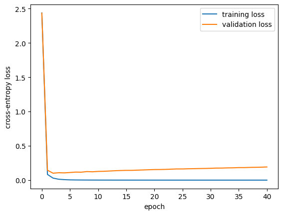
We train with cell_type as the target and cross-entropy loss. The training and validation curves show learning progress.

n_classes = len(adata.obs["cell_type"].cat.categories)
clf_model, train_losses, val_losses = train_model(
    "cell_type", kind="classification", n_out=n_classes, loss_fn=nn.CrossEntropyLoss(),
)

epochs = np.arange(len(train_losses))
plt.plot(epochs, train_losses, label="training loss")
plt.plot(epochs, val_losses, label="validation loss")
plt.xlabel("epoch")
plt.ylabel("cross-entropy loss")
plt.legend()
plt.show()

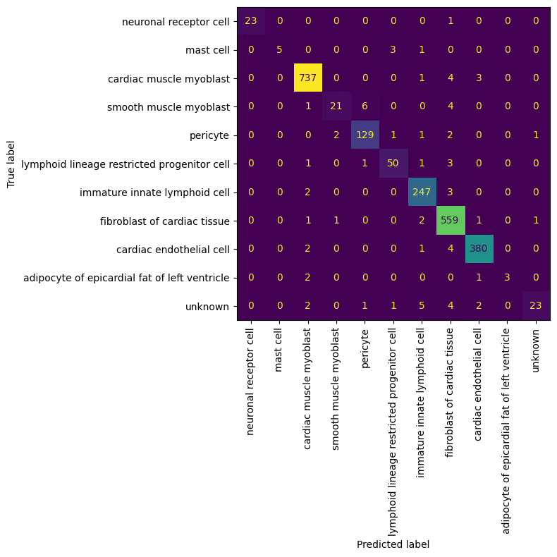
On the held-out test cells we report accuracy and a confusion matrix, which shows which cell types the model mixes up.

test = next(iter(AnnLoader(adata[test_idx], batch_size=len(test_idx))))
clf_model.eval()
with torch.no_grad():
    preds = clf_model(test.X.to(device)).argmax(dim=1).cpu().numpy()
truth = test.obs["cell_type"].cat.codes.to_numpy(copy=True)

print(f"test accuracy: {(preds == truth).mean():.2f}")

class_names = list(adata.obs["cell_type"].cat.categories)
disp = ConfusionMatrixDisplay.from_predictions(
    truth, preds, labels=range(len(class_names)), display_labels=class_names,
    xticks_rotation="vertical", colorbar=False,
)
disp.figure_.set_size_inches(8, 8)
plt.tight_layout()
plt.show()

test accuracy: 0.97

Example 2: predicting a continuous property

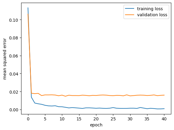
Changing task means changing one thing: the target column. Here we predict percent_mito, the fraction of a cell’s counts that come from mitochondrial genes, a common continuous quality score. We pass kind="regression", train the same network with a single output and mean-squared-error loss, and reuse the same split and helper.

reg_model, train_losses, val_losses = train_model(
    "percent_mito", kind="regression", n_out=1, loss_fn=nn.MSELoss(),
)

epochs = np.arange(len(train_losses))
plt.plot(epochs, train_losses, label="training loss")
plt.plot(epochs, val_losses, label="validation loss")
plt.xlabel("epoch")
plt.ylabel("mean squared error")
plt.legend()
plt.show()

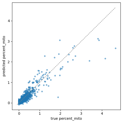
We score the regression with R2, the share of the variation the model captures, where 1.0 is perfect, and plot predicted against true values. Points on the dashed line are exact.

test = next(iter(AnnLoader(adata[test_idx], batch_size=len(test_idx))))
reg_model.eval()
with torch.no_grad():
    pred = reg_model(test.X.to(device)).cpu().view(-1).numpy()
truth = test.obs["percent_mito"].cpu().numpy()

print(f"test R^2: {r2_score(truth, pred):.2f}")

fig, ax = plt.subplots(figsize=(5, 5))
ax.scatter(truth, pred, s=12, alpha=0.5)
lims = [min(truth.min(), pred.min()), max(truth.max(), pred.max())]
ax.plot(lims, lims, color="grey", linestyle="--", linewidth=1)
ax.set_xlabel("true percent_mito")
ax.set_ylabel("predicted percent_mito")
plt.tight_layout()
plt.show()

test R^2: 0.85

Recap and next step

AnnLoader hands the training loop batches straight from the AnnData object, and switching between classification and regression was a one-line change of the target column: one cell in, one label out.

Some tasks do not fit that shape. When one training example is a whole patient, all of a donor’s cells with a single group label, a per-cell loader cannot express it, but the same Dataset interface can. That is the subject of the next tutorial, Patient-level learning.